The primary function HDStIM() in the HDStIM
package follows a heuristic approach to group cells into responding and
non-responding. For a combination of cell population and stimulation
type (e.g., CD127+ T-helper cells and interferon-alpha),
HDStIM() starts by performing K-means clustering on the
combined set of cells from stimulated and unstimulated samples. K-means
clustering is performed on combined expression data of all the state
(signaling/intracellular) markers. Upon clustering using a contingency
table as shown below, a Fisher’s exact test determines the effect size
and the statistical significance of partitioning. Cells from the
combinations that pass the Fisher’s exact test (p-value < 0.05) are
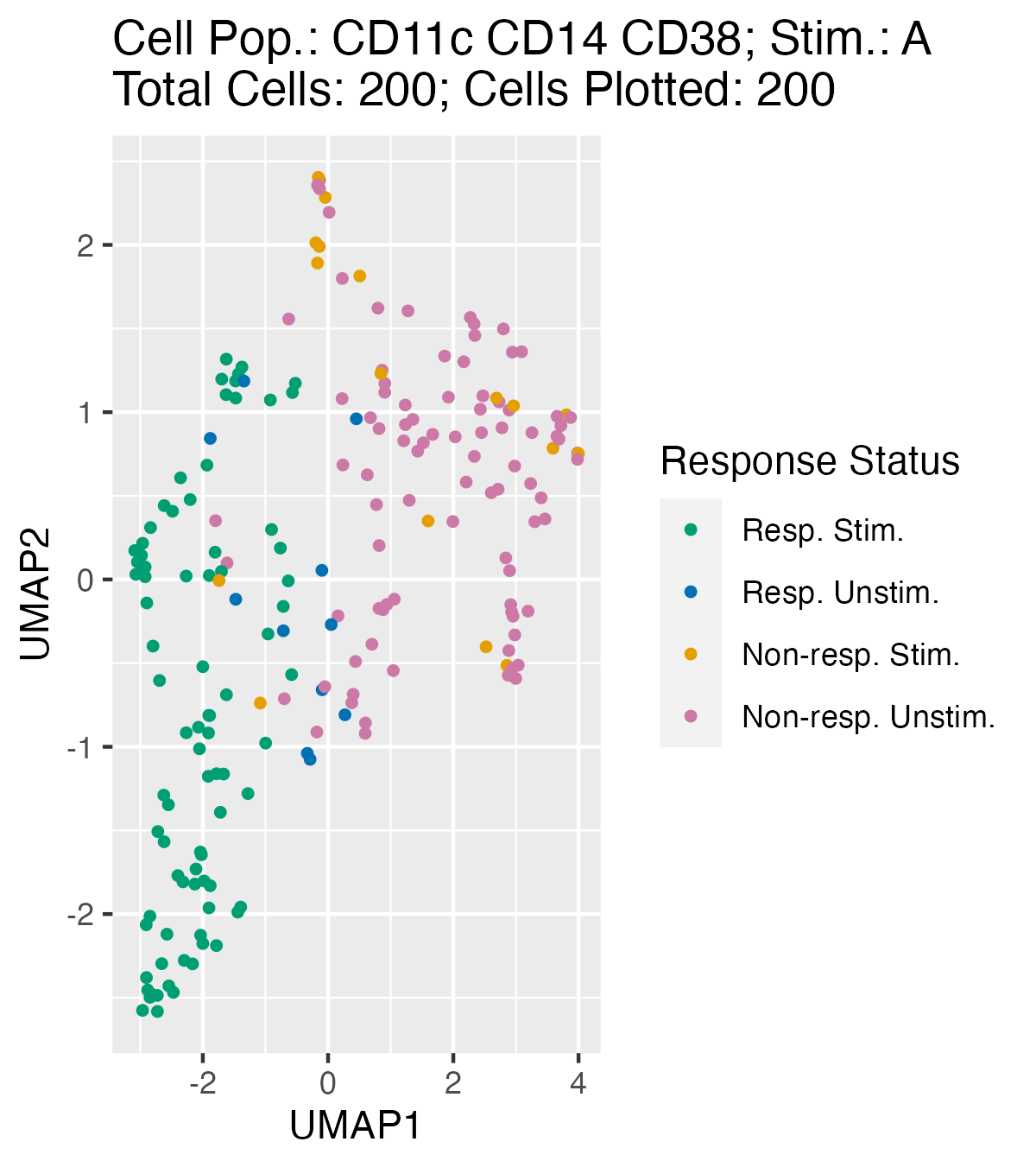
considered responding. An optional UMAP can also be calculated to
visually verify the cell partitioning in responding and non-responding
groups by using auxiliary plotting scripts provided in the package.
In addition to an auxiliary script to plot UMAPs, the package also comes with two other plotting scripts for K-means clustering and Fisher’s exact test and state marker density before and after mapping.
An example of the contingency table used for Fisher’s exact test.
matrix(c(60, 40, 20, 80),nrow = 2, ncol = 2,
       dimnames = list(c("Cluster1", "Cluster2"), c("Stim", "Unstim")))
#>          Stim Unstim
#> Cluster1   60     20
#> Cluster2   40     80
To Run The Main HDStIM Function
As stated above, HDStIM() is the primary function of the
HDStIM package. We will use the example data set
chi11 (from mass cytometry) included in the package.
Note:chi11 is a minimal dataset included for unit
testing only. Therefore, it does not represent a typical mass/flow
cytometry assay.
library(HDStIM)

mapped_data <-  HDStIM(chi11$expr_data, chi11$state_markers,
                       chi11$cluster_col, chi11$stim_label,
                       chi11$unstim_label, seed_val = 123,
                       umap = TRUE, umap_cells = 500,
                       verbose = FALSE)

class(mapped_data)
#> [1] "list"

attributes(mapped_data)
#> $names
#>  [1] "response_mapping_main" "stacked_bar_plot_data" "state_markers"
#>  [4] "cellpop_col"           "stim_label"            "unstim_label"
#>  [7] "seed_val"              "all_fisher_p_val"      "all_k_means_data"
#> [10] "umap_plot_data"        "umap"                  "umap_cells"
Output
HDStIM() returns a list with the mapped expression data,
data to plot stacked bar plots to visualize the K-means and Fisher’s
exact test results, and data to plot the optional UMAPs. The list also
includes tables containing statistical information from K-means and
Fisher’s exact test and other information passed as the function
attributes.
head(mapped_data$response_mapping_main)
#> # A tibble: 6 × 41
#>   cluster_id sample_id      condition patient_id stim_type cell_population  CD45
#>        <dbl> <chr>          <chr>     <chr>      <chr>     <chr>           <dbl>
#> 1         79 CHI-011_1_2_G  CHI       CHI-011    G         CD11c CD14 CD38  3.48
#> 2         69 CHI-011_2_4_G  CHI       CHI-011    G         CD11c CD14 CD38  2.22
#> 3         69 CHI-011_4_13_G CHI       CHI-011    G         CD11c CD14 CD38  3.03
#> 4         79 CHI-011_4_11_G CHI       CHI-011    G         CD11c CD14 CD38  2.82
#> 5         69 CHI-011_2_5_G  CHI       CHI-011    G         CD11c CD14 CD38  2.07
#> 6         69 CHI-011_1_1_G  CHI       CHI-011    G         CD11c CD14 CD38  3.39
#> # ℹ 34 more variables: CD7 <dbl>, CD19 <dbl>, pPLCg2 <dbl>, CD4 <dbl>,
#> #   IgD <dbl>, CD20 <dbl>, CD25 <dbl>, pSTAT5 <dbl>, CD123 <dbl>, AKT <dbl>,
#> #   pSTAT1 <dbl>, CD27 <dbl>, pP38 <dbl>, CD24 <dbl>, pSTAT3 <dbl>,
#> #   CD11c <dbl>, CD14 <dbl>, CD56 <dbl>, IkBa <dbl>, pCREB <dbl>, CD16 <dbl>,
#> #   CD38 <dbl>, CD8 <dbl>, CD45RA <dbl>, CD3 <dbl>, pERK1_2 <dbl>,
#> #   HLA_DR <dbl>, pS6 <dbl>, CD127 <dbl>, ncount <int>, k_cluster_id <int>,
#> #   responding_cluster <int>, response_status <chr>, comb_no <int>
head(mapped_data$stacked_bar_plot_data)
#> # A tibble: 6 × 7
#>   cell_population            stim_type  f_p_val stim_clust stim_status k_cluster
#>   <chr>                      <chr>        <dbl>      <dbl> <chr>       <chr>
#> 1 CD11c CD14 CD38            A         3.05e-26          1 unstim      cluster1
#> 2 CD11c CD14 CD38            A         3.05e-26          1 unstim      cluster2
#> 3 CD11c CD14 CD38            A         3.05e-26          1 stim        cluster1
#> 4 CD11c CD14 CD38            A         3.05e-26          1 stim        cluster2
#> 5 CD19 CD20 CD45RA HLA-DR C… A         5.56e-18          2 unstim      cluster1
#> 6 CD19 CD20 CD45RA HLA-DR C… A         5.56e-18          2 unstim      cluster2
#> # ℹ 1 more variable: cell_count_perc <dbl>
head(mapped_data$umap_plot_data)
#> # A tibble: 6 × 8
#>   cell_population stim_type condition tot_of_cells no_of_cells  UMAP1  UMAP2
#>   <chr>           <chr>     <chr>     <chr>        <chr>        <dbl>  <dbl>
#> 1 CD11c CD14 CD38 A         CHI       200          200          0.938 -0.149
#> 2 CD11c CD14 CD38 A         CHI       200          200          1.92   1.09
#> 3 CD11c CD14 CD38 A         CHI       200          200         -1.91  -0.812
#> 4 CD11c CD14 CD38 A         CHI       200          200          0.773  0.447
#> 5 CD11c CD14 CD38 A         CHI       200          200          1.24   0.926
#> 6 CD11c CD14 CD38 A         CHI       200          200         -1.48   1.08
#> # ℹ 1 more variable: response_status <chr>
head(mapped_data$all_fisher_p_val)
#>   stim_type              cell_population stim_clust1 stim_clust2 unstim_clust1
#> 1         A              CD11c CD14 CD38          83          17            11
#> 2         A                 CD11c HLA-DR          43          57            50
#> 3         A CD19 CD20 CD45RA HLA-DR CD24          23          77            83
#> 4         A               CD3 CD27 CD127          35          65            32
#> 5         A          CD3 CD4 CD27 CD45RA          34          66            42
#> 6         A               CD3 CD4 HLA-DR          37          63            39
#>   unstim_clust2    estimate      p.value    conf.low  conf.high
#> 1            89 38.31592946 3.052288e-26 16.41025641 97.9574110
#> 2            50  0.75546384 3.950464e-01  0.41598165  1.3672058
#> 3            17  0.06232828 5.555794e-18  0.02850666  0.1296101
#> 4            68  1.14345766 7.645958e-01  0.60968684  2.1500051
#> 5            58  0.71262870 3.078444e-01  0.38474999  1.3129671
#> 6            61  0.91899062 8.842353e-01  0.49842428  1.6921035
#>                               method alternative      f_p_adj
#> 1 Fisher's Exact Test for Count Data   two.sided 2.441830e-25
#> 2 Fisher's Exact Test for Count Data   two.sided 7.023047e-01
#> 3 Fisher's Exact Test for Count Data   two.sided 2.539791e-17
#> 4 Fisher's Exact Test for Count Data   two.sided 9.212285e-01
#> 5 Fisher's Exact Test for Count Data   two.sided 6.156888e-01
#> 6 Fisher's Exact Test for Count Data   two.sided 9.781822e-01
head(mapped_data$all_k_means_data)
#>   stim_type              cell_population    pPLCg2    pSTAT5        AKT
#> 1         A              CD11c CD14 CD38 0.6036923 1.5150197 0.19882950
#> 2         A              CD11c CD14 CD38 0.3433208 0.5100987 0.14467489
#> 3         A                 CD11c HLA-DR 0.2754466 0.2628448 0.08187613
#> 4         A                 CD11c HLA-DR 0.9878153 0.5947371 0.10871637
#> 5         A CD19 CD20 CD45RA HLA-DR CD24 0.2804838 0.2853633 0.07871608
#> 6         A CD19 CD20 CD45RA HLA-DR CD24 0.3600085 1.9650785 0.12718000
#>       pSTAT1       pP38    pSTAT3      IkBa    pCREB    pERK1_2        pS6 size
#> 1 2.46662032 0.85286553 1.4007937 1.8315034 2.752456 0.10329694 0.27964780   94
#> 2 0.80050991 0.69575908 0.2100968 1.4439438 2.346255 0.04306572 0.16080807  106
#> 3 0.09136274 0.03271188 0.0532651 0.8501084 0.437598 0.03960397 0.07132055   93
#> 4 0.65155894 0.13219535 0.2322881 2.4118800 2.118350 0.02017302 0.12388073  107
#> 5 0.51540424 0.12034285 0.1396368 2.7656495 1.401279 0.13669583 0.10065605  106
#> 6 1.79297154 0.21265052 0.7480344 3.1434614 1.702514 0.20580153 0.18568148   94
#>   withinss cluster
#> 1 342.6724       1
#> 2 340.0997       2
#> 3 174.5916       1
#> 4 266.5471       2
#> 5 255.0538       1
#> 6 236.2004       2
To Plot Diagnostic Figures
Plots Explaining K-means Clustering And Fisher’s Exact Test
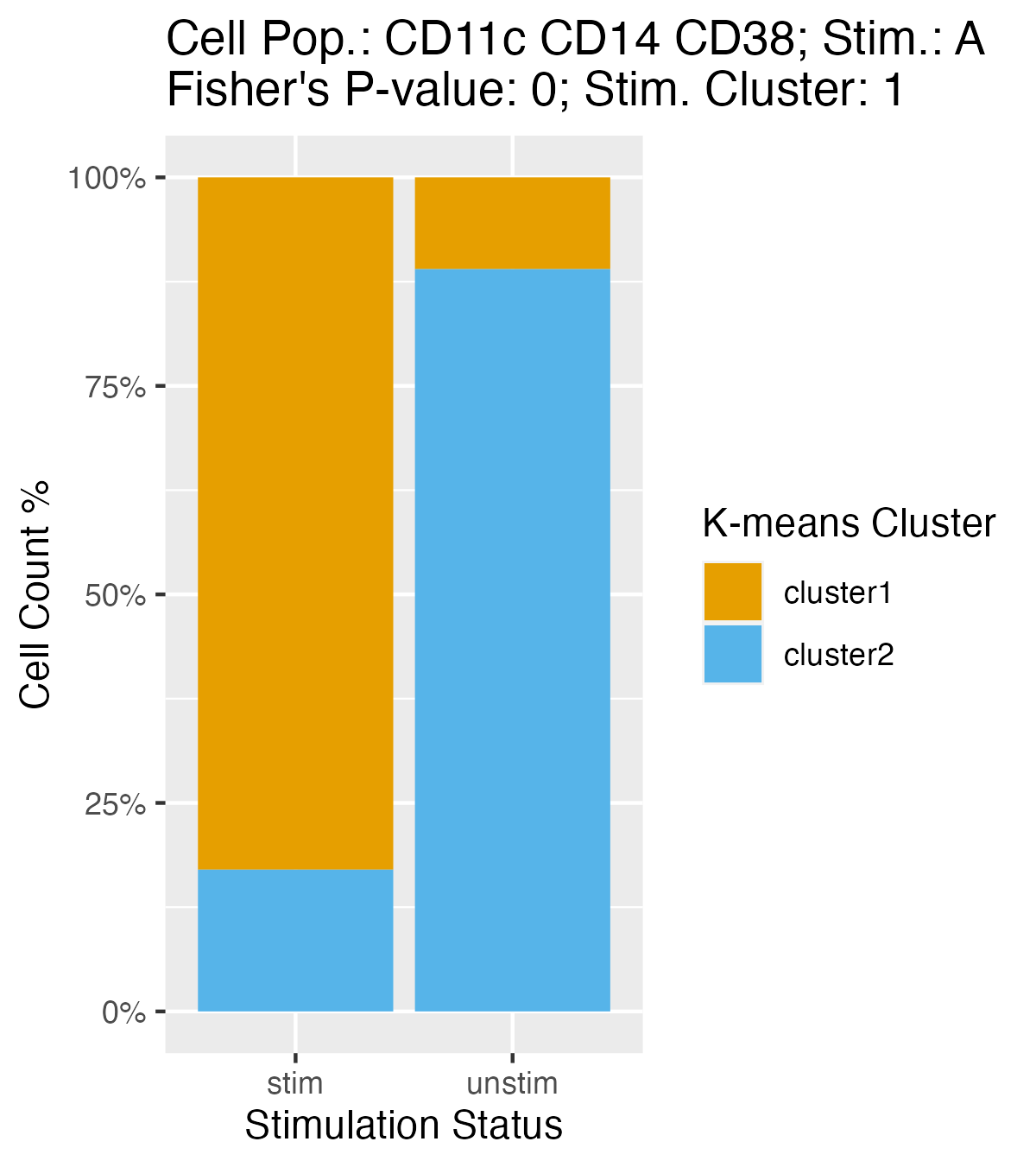
Using the stacked_bar_plot_data,
plot_K_Fisher() generates bar plots showing the percentage
of cells from the stimulated and unstimulated samples clustered in the
two K-means clusters a given cell population and stimulation type.
plot_K_Fisher() returns a list of ggplot objects. If the
path is specified, it can also render and save the plots in PNG
format.
k_plots <- plot_K_Fisher(mapped_data, path = NULL, verbose = FALSE)
k_plots[[1]]
UMAP Plots To Visually Inspect Responding and Non-Responding Cell Mapping
Note: You can only generate these plots if you have asked UMAPs
to be calculated in the HDStIM() function.
UMAP plots can be helpful for visually inspecting how well
HDStIM() has mapped responding vs. non-responding cells for
a cell population and stimulation type. plot_umap() also
returns a list of ggplot objects and if the path is specified, it will
render and save the plots in PNG format.
u_plots <- plot_umap(mapped_data, path = NULL, verbose = FALSE)
u_plots[[1]]
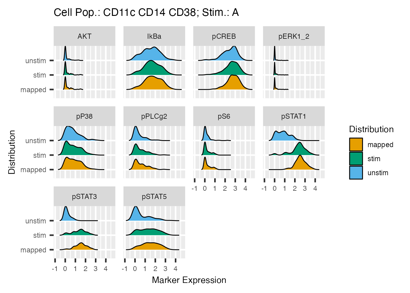
Distribution Plots for Individual State Marker before And After Mapping
For each state/signaling markers distribution plots shows the kernel
density estimation of the pre HDStIM() data from both
stimulated and unstimulated samples along with the density from cells
from stimulated samples mapped as responding. plot_exprs()
also returns a list of ggplot objects and if the path is specified, it
will render and save the plots in PNG format.
e_plots <- plot_exprs(mapped_data, path = NULL,verbose = FALSE)
library(ggplot2)
e_plots[[1]] +
    theme(text = element_text(size = 11))
#> Picking joint bandwidth of 0.0611
#> Picking joint bandwidth of 0.274
#> Picking joint bandwidth of 0.21
#> Picking joint bandwidth of 0.0301
#> Picking joint bandwidth of 0.23
#> Picking joint bandwidth of 0.191
#> Picking joint bandwidth of 0.102
#> Picking joint bandwidth of 0.179
#> Picking joint bandwidth of 0.172
#> Picking joint bandwidth of 0.288
To Rank State/Signaling Markers According To Their Contribution To The Response
marker_ranking_boruta() function runs Boruta on the
stimulation - cell population combinations that passed the Fisher’s
exact test to rank the markers according to their contribution to the
response. The function returns a list with a tibble containing attribute
statistics calculated by Boruta and ggplot objects. If the path is not
NULL, plots are also rendered and saved in the specified folder in PNG
format.
m_ranks <- marker_ranking_boruta(mapped_data, path = NULL, n_cells = NULL,
                                 max_runs = 100, seed_val = 123,
                                 verbose = FALSE)

head(m_ranks$attribute_stats)
#> # A tibble: 6 × 9
#>   stim_type cell_population state_marker meanImp medianImp minImp maxImp
#>   <chr>     <chr>           <fct>          <dbl>     <dbl>  <dbl>  <dbl>
#> 1 A         CD11c CD14 CD38 pP38          0.0606     0.109 -1.46    2.07
#> 2 A         CD11c CD14 CD38 AKT           0.0420     0.197 -1.87    1.60
#> 3 A         CD11c CD14 CD38 pERK1_2       2.50       2.66  -0.690   4.92
#> 4 A         CD11c CD14 CD38 pPLCg2        2.87       2.80   0.719   5.10
#> 5 A         CD11c CD14 CD38 pS6           2.75       2.90   0.229   4.99
#> 6 A         CD11c CD14 CD38 pCREB         4.52       4.44   2.04    7.26
#> # ℹ 2 more variables: normHits <dbl>, decision <chr>

m_ranks$plots[[1]]